Interactive Exercises for R and tidyverse: Was Chivalry Dead on the Titanic?
Companion Exercises for Practical Machine Learning with R
NotePlease be Patient: Loading R Environment
The interactive R environment and the required packages must be loaded in your browser. This typically takes 1–2 minutes. You can monitor the progress in the bottom-right corner.
When everything is loaded, you get a “Ready to roll” message below. Thank you for your patience!
1 Introduction:
In this interactive section, you will work on a small project to determine if chivalry was dead when the Titanic sank in 1912. The background for the project is an article written by Hannah Furness (Royal Correspondent at The Telegraph). She cites a Swedish historian claiming, “It was ‘not true’ that women and children on board the Titanic survived thanks to the gallantry of men.” Hannah Furness also reports anecdotal evidence about men being in the lifeboats instead of women: “Over on the starboard side, it was a different story. On the last boats to leave, the majority were men.”However, Furness did not use any statistics to support her claim, although data are publicly available.
It is now your job to fill this gap. The question is:
Was the proportion of women surviving the Titanic disaster greater than the one of men?
If true, that would strongly indicate that the ultimate chivalry — dying to protect a woman’s life — was still present when the Titanic sank and that Furness’ claim that chivalry was dead in 1912 is likely incorrect.
2 Analyzing Titanic Survival Rates for Women and Men
You will use the same Titanic dataset we used before together with the tidyverse package (already loaded in the background). The Titanic dataset contains 887 observations about Titanic passengers, including variables such as a survival indicator, passenger’s sex, and the class traveled in. The dataset covers about 67% of the total passengers from the Titanic.
Below are the first six observations from the DataTitanic data frame:
  Survived Pclass                        Name    Sex Age SiblingsSpousesAboard
1        0      3      Mr. Owen Harris Braund   male  22                     1
2        1      1   Mrs. John Bradley Cumings female  38                     1
3        1      3       Miss. Laina Heikkinen female  26                     0
4        1      1 Mrs. Jacques Heath Futrelle female  35                     1
5        0      3     Mr. William Henry Allen   male  35                     0
6        0      3             Mr. James Moran   male  27                     0
  ParentsChildrenAboard FareInPounds
1                     0       7.2500
2                     0      71.2833
3                     0       7.9250
4                     0      53.1000
5                     0       8.0500
6                     0       8.4583
Before writing R code, we need to develop a data analysis strategy:
- Step 1:
-
You will create a data frame,
DataAnalysis, containing only the variablesSurvived,Sex,Pclass. In addition, you will transform the variableSurvivedto a logic variable withTRUEandFALSEvalues, and you will renamePclasstoPasClass. - Step 2:
-
You will divide the data frame
DataAnalysisinto two new data frames,DataWomenandDataMen,containing only observations for women and men, respectively. - Step 3:
-
The data frames
DataWomenandDataMenwill finally be used to calculate the survival rates of women and men.
Remember, whenever you work on a data science project, develop a detailed data analysis strategy before you start coding. Otherwise, after you have spent a lot of time coding, you might need to entirely change your code because you forgot to consider an important fact.
You will now follow the steps outlined above to write the R code for the project.
Step 1 from the data analysis strategy requires to create a new data frame DataAnalysis that only contains the variables Survived (as logic data type), Sex, and Pclass (renamed to PasClass).
When you substitute the ______ in the code below, the command head(DataAnalysis) will print the first six observations of the new data frame to the console (note that the data frame DataTitanic has already been loaded in the background):
Here is a hint:
Use the select() command and list the variables (columns) that you like to have included in the new data frame. Make sure to rename Pclass to PasClass.
The mutate() command to convert the variable Survived from numeric to logic is already provided.
Here is the solution:
DataAnalysis=DataTitanic |>
               select(Survived,Sex,PasClass=Pclass) |> #<1>
               mutate(Survived=as.logical(Survived))   #<2>
head(DataAnalysis)
- 1
-
In the
select()command you list the variables you like to use. SincePclassin the Titanic dataset will be renamed toPasClass, you writePasClass=Pclass. - 2
-
the
as.logical()command converts a variable such as a \(0\) and \(1\) variable to alogicalvariable withTRUEandFALSEvalues.
Step 2 from the data analysis strategy requires splitting the data frame DataAnalysis into two data frames:
DataWomenshould only contain female passengers.DataMenshould only contain male passengers.
In the code block below you can use the filter() command to generate the two new data frames:
Here is a hint:
The two filter() commands each need a condition for the observations to be filtered.
Add the variable name left of the == and the filter-value right of the == (do not forget the quotes).
Here is the solution
DataWomen=DataAnalysis |>
          filter(Sex=="female") #<1>
DataMen=DataAnalysis |>
          filter(Sex=="male") #<2>
head(DataWomen)
head(DataMen)

1. The new data frame `DataWomen` will only contain observations where `Sex=="female"`
2. The new data frame `DataMen` will only contain observations where `Sex=="male"`
DataWomen=DataAnalysis |>
          filter(Sex=="female")
DataMen=DataAnalysis |>
          filter(Sex=="male")
head(DataWomen)
head(DataMen)

1. The new data frame `DataWomen` will only contain observations where `Sex=="female"`
2. The new data frame `DataMen` will only contain observations where `Sex=="male"`
Now that you have two different data frames that either only contain male or female passengers’ observations, you are ready to calculate the related survival rates.
In the code block below, you will calculate the female survival rate. Later, for the male survival rate, we will show you a shorter alternative.
The female survival rate \((Fem_{SurvRate})\) is defined as:
\[Fem_{SurvRate}=\frac{\mbox{Count of female survivors}}{\mbox{Count of all females}}\]
Therefore, to calculate the female survival rate, you need to find the number of female passengers that survived \((Fem_{Surv})\) and the total number of female passengers \(Fem_{Total}\). The latter is the same as the number of observations in the data frame DataWomen and can be calculated with nrow(DataWomen).
To find the number of surviving women \((Fem_{Surv})\), we can use the fact that a surviving passenger was coded with TRUE with an internal value of \(1\) and a not-surviving passenger with FALSE with an internal value of \(0\). Therefore, when we extract the variable \(Survived\) as a vector-object from the data frame ‘DataWomen’ and calculate the sum from this vector, we get the number of female survivors (sum(DataWomen$Survived)).
With this information, you should be ready to complete the code below to calculate the rate of female survivors (note that the data frame DataWomen has been loaded already in the background):
Here is a hint:
The female survival rate is calculated by dividing the number of female survivors by the total number of female passengers.
The sum of the variable Survived in the data frame DataWomen gives you the number of female survivors (why?).
The number of female passengers is the same as the number of observations in the data frame DataWomen, which you can get with the command nrow().
Here is the Solution
FemSurv=sum(DataWomen$Survived)
FemTotal=nrow(DataWomen)
FemSurvRate= FemSurv/FemTotal
cat("The survival rate for women is",FemSurvRate)
FemSurv=sum(DataWomen$Survived)
FemTotal=nrow(DataWomen)
FemSurvRate= FemSurv/FemTotal
cat("The survival rate for women is",FemSurvRate)
You could do the same for the male passengers. However, there is a shorter alternative to calculate the male survival rate:
Why could the mean() command be used to calculate the survival rate directly? It is because the mean is calculated by dividing the sum of a variable by the number of observations. This is what we did explicitly when we calculated the female survival rate.
When we use the cat() command again to print and compare the female and male survival rates next to each other, you can see that the survival rate for female passengers is much higher than the one for male passengers:
The remaining question is if the difference between the two survival rates is high enough to allow us to reject the assertion of the Telegraph article that chivalry was dead in 1912?
To answer this question, we need more analysis. R really shines when data are well organized, as done here — when good data engineering is performed. With the prop.test() command, R can run a test if the survival rates for women and men differ significantly. The syntax only requires the values for four arguments:
the number of female survivors,
the number of male survivors,
the number of total female passengers, and
the number of total male passengers.
These values have been calculated already and stored in the R Objects WomenSurv, MenSurv, WomenTotal, and MenTotal. We can provide these values to the prop.test() command grouped as two R vectors, one for the survival numbers and one for the total numbers for women and men, respectively:
Below, we saved the output of the prop.test() command in an R object named ModelPropFemaleVsMale. We started the object name with the word Model to indicate that it stores the output of a statistical model. ModelPropFemaleVsMale is a complex object. However, when we print it with the print() command, we extract important information from the model object:
Reading the output above backward, starting with the last line, allows us to develop the final result step by step. The last line from the ModelPropFemaleVsMale object shows the different survival rates for female (Prop1) and male (Prop2) passengers. The difference between these two survival rates is about 0.55. The 95%-confidence interval for the difference ranges from 0.49 to 0.61. The probability of this difference being zero (both survival rates would be the same) is expressed by the P-value in line five of the output. As the P-value shows, the probability for the female and the male survival rate to be the same is almost zero.
We can summarize:
The assertion from the Telegraph that chivalry was dead in 1912 during the Titanic disaster is most likely not correct.
3 Backdoor Effects and Confounder PasClass
Our previous analysis contains a significant logical oversight, illustrated in the causal graph below:
Code
library(ggdag)
library(ggplot2)
set.seed(123)
dagify(
  Survived ~ Sex + PClass,
  Sex ~ PClass,
  exposure = "Sex",
  outcome = "Survived"
) |>
  ggdag_status(node_size = 22) +
  theme_void()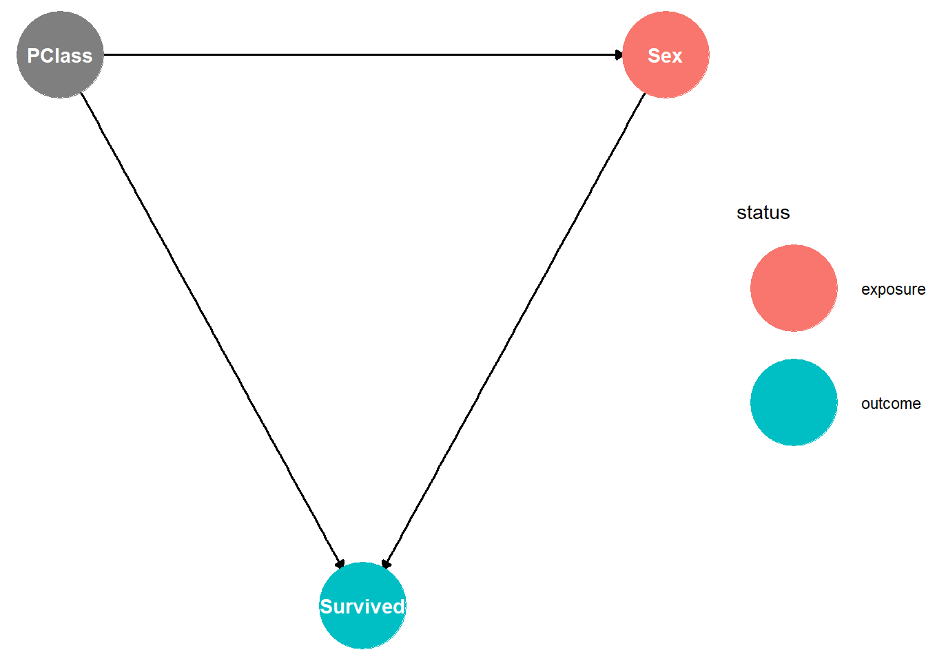
Passengers in third class, located in the lower decks of the Titanic, had much lower survival rates than others. Additionally, third class had a higher proportion of men, as it was primarily comprised of emigrants — many of whom were single men rather than single women.
Looking at the graph, the variable Sex influences survival in two distinct ways:
Directly: This represents the effect we want to measure (the impact of chivalry/social norms).
Indirectly (Backdoor Effect): Because third class was both deadlier and predominantly male, it lowers the overall survival average for men regardless of chivalry. In this context, the variable
PClassis called a confounder.
Consequently, the direct relationship is not being measured accurately. To close the backdoor, we must control for PClass. One method is to run the analysis separately for each passenger class. By only considering a single class, the correlation between PClass and Sex no longer impacts the outcome, effectively closing the backdoor path.
3.1 Closing the Backdoor Path: Analyzing only First Class Passengers
We will begin by analyzing first-class passengers only. The code from the previous exercise is provided below; you simply need to add two filter() commands for the male and female data frames to ensure the dataset only include passengers from the first class.
For your convenience the code from the previous section is already copied to be amended with the two filter() commands:
Add two filter() commands, one to each pipe and do not forget the piping symbol |>. The condition for the filter would be PasClass==1.
Here is the solution:
DataWomen=DataAnalysis |>
          filter(Sex=="female") |>
          filter(PasClass==1) #<1>
DataMen=DataAnalysis |>
          filter(Sex=="male") |>
          filter(PasClass==1) #<2>

MaleSurvRate= mean(DataMen$Survived)
FemSurvRate= mean(DataWomen$Survived)

cat("The survival rate for women in this class is:", FemSurvRate, "\n",
    "The survival rate for men in this class is:", MaleSurvRate )
DataWomen=DataAnalysis |>
          filter(Sex=="female") |>
1          filter(PasClass==1)
DataMen=DataAnalysis |>
          filter(Sex=="male") |>
2          filter(PasClass==1)

MaleSurvRate= mean(DataMen$Survived)
FemSurvRate= mean(DataWomen$Survived)

cat("The survival rate for women in this class is:", FemSurvRate, "\n",
"The survival rate for men in this class is:", MaleSurvRate )- 1
-
Here is the extra
filter()command to ensure only first class passengers for the female dataset are considered. - 2
-
Here is the extra
filter()command to ensure only first class passengers for the for the male dataset are considered.
3.2 Closing the Backdoor Path: Analyzing only Second Class Passengers
We will now only analyze second-class passengers.
Copy the code from the previous section and adjust it to ensure the code applies to the second class rather than the first class.
Ensure that the two commands that filter for passenger class, do filter for the correct class.
Here is the solution:
DataWomen=DataAnalysis |>
          filter(Sex=="female") |>
          filter(PasClass==2) #<1>
DataMen=DataAnalysis |>
          filter(Sex=="male") |>
          filter(PasClass==2) #<2>

MaleSurvRate= mean(DataMen$Survived)
FemSurvRate= mean(DataWomen$Survived)

cat("The survival rate for women in this class is:", FemSurvRate, "\n",
    "The survival rate for men in this class is:", MaleSurvRate )
DataWomen=DataAnalysis |>
          filter(Sex=="female") |>
1          filter(PasClass==2)
DataMen=DataAnalysis |>
          filter(Sex=="male") |>
2          filter(PasClass==2)

MaleSurvRate= mean(DataMen$Survived)
FemSurvRate= mean(DataWomen$Survived)

cat("The survival rate for women in this class is:", FemSurvRate, "\n",
"The survival rate for men in this class is:", MaleSurvRate )- 1
-
For the pipe that defines
DataWomen, here is the place where you must changePasClass==1toPasClass==2. - 2
-
For the pipe that defines
DataMen, here is the place where you must changePasClass==1toPasClass==2.
3.3 Closing the Backdoor Path: Analyzing only Third Class Passengers
We will now only analyze third-class passengers.
Copy the code from the previous section and adjust it to ensure the code applies to the third class rather than the second class.
Ensure that the two commands that filter for passenger class, do filter for the correct class.
Here is the solution:
DataWomen=DataAnalysis |>
          filter(Sex=="female") |>
          filter(PasClass==3) #<1>
DataMen=DataAnalysis |>
          filter(Sex=="male") |>
          filter(PasClass==3) #<2>

MaleSurvRate= mean(DataMen$Survived)
FemSurvRate= mean(DataWomen$Survived)

cat("The survival rate for women in this class is:", FemSurvRate, "\n",
    "The survival rate for men in this class is:", MaleSurvRate )
DataWomen=DataAnalysis |>
          filter(Sex=="female") |>
1          filter(PasClass==3)
DataMen=DataAnalysis |>
          filter(Sex=="male") |>
2          filter(PasClass==3)

MaleSurvRate= mean(DataMen$Survived)
FemSurvRate= mean(DataWomen$Survived)

cat("The survival rate for women in this class is:", FemSurvRate, "\n",
"The survival rate for men in this class is:", MaleSurvRate )- 1
-
For the pipe that defines
DataWomen, here is the place where you must changePasClass==2toPasClass==3. - 2
-
For the pipe that defines
DataMen, here is the place where you must changePasClass==2toPasClass==3.
Happy Analytics!