Tree Based Models
Decision Trees
Introduction
Decision Trees can be used for
- Classification
- Regression
Decision Trees can be used as standalone algorithms (this is what we do here)
Decision Trees can be used as components for other models such as:
- Random Forest Models
- Boosted Tree Models
Introducing the Idea of Decision Trees with the Titanic Dataset
Code
library(rio); library(tidymodels); library(janitor)
library(kableExtra)
DataTitanic=import("https://ai.lange-analytics.com/data/Titanic.csv") %>%
            clean_names("upper_camel") %>%
             select(Survived, Sex, Class=Pclass, Sex, Age, Fare=FareInPounds) %>%
             mutate(Survived=as.factor(Survived))

set.seed(777)
Split7525=initial_split(DataTitanic, strata = Survived)

DataTrain=training(Split7525)
DataTest=testing(Split7525)

kbl(DataTrain[1:5,])| Survived | Sex | Class | Age | Fare |
|---|---|---|---|---|
| 0 | male | 3 | 35 | 8.0500 |
| 0 | male | 1 | 54 | 51.8625 |
| 0 | male | 3 | 2 | 21.0750 |
| 0 | male | 3 | 20 | 8.0500 |
| 0 | male | 3 | 39 | 31.2750 |
Generating a Decision Tree with tidymodels
Note, rpart package needs to be installed. tidymodels loads the rpart package automatically. Therefore library(rpart) is not needed.
Code
══ Workflow [trained] ══════════════════════════════════════════════════════════
Preprocessor: Recipe
Model: decision_tree()

── Preprocessor ────────────────────────────────────────────────────────────────
0 Recipe Steps

── Model ───────────────────────────────────────────────────────────────────────
n= 664

node), split, n, loss, yval, (yprob)
      * denotes terminal node

 1) root 664 256 0 (0.61445783 0.38554217)
   2) Sex=male 428  84 0 (0.80373832 0.19626168)
     4) Age>=13 400  68 0 (0.83000000 0.17000000) *
     5) Age< 13 28  12 1 (0.42857143 0.57142857)
      10) Class>=2.5 20   8 0 (0.60000000 0.40000000) *
      11) Class< 2.5 8   0 1 (0.00000000 1.00000000) *
   3) Sex=female 236  64 1 (0.27118644 0.72881356)
     6) Class>=2.5 114  56 0 (0.50877193 0.49122807)
      12) Fare>=23.35 22   1 0 (0.95454545 0.04545455) *
      13) Fare< 23.35 92  37 1 (0.40217391 0.59782609) *
     7) Class< 2.5 122   6 1 (0.04918033 0.95081967) *
Displaying the Decision Tree with rpart.plot
Note, rpart.plot package needs to be installed and loaded with library(rpart.plot).

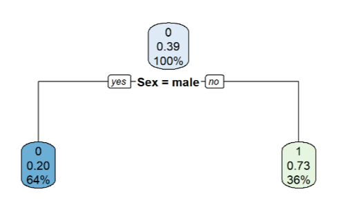
Nodes in the Decision Tree (ignore decision rules for now)

- Nodes are like containers holding all or some of the training data
- root node holds all training observations.
- moving down the tree parent nodes get split into child nodes
RPartnodes show three types of information.»
Nodes in the Decision Tree — The Optimizer Created Decision Rules
Let us follow the last observation in DataTrain
| Survived | Sex | Class | Age | Fare | |
|---|---|---|---|---|---|
| 664 | 1 | male | 1 | 26 | 30 |

Nodes in the Decision Tree — Interpreting Terminal Nodes

Nodes in the Decision Tree — Stylized Facts

Adult male passengers, regardless of the class and fare, had only a survival rate of 17%.
Female passengers, regardless of age and not considering the class or the fare, had a survival chance of 73%.
Considering the class female passengers traveled in (regardless of age), the survival rate was 95% for First or Second Class.
Nodes in the Decision Tree — Not all Decision Rules Make Sense

For example:
Females traveling in Third Class have a survival rate of 49% (this makes sense)
Next split does not make much sense:
- Fare greater or equal to 23 British Pounds survival rate only 5%.
- In contrast, lower fare had a survival rate of 60%.»
Predicting Testing Data with a Decision Tree

| Survived | Sex | Class | Age | Fare |
|---|---|---|---|---|
| 1 | male | 3 | 9 | 15.9 |
Prediction: Not Survived
Observation is a false positive (0=:positive class)»
Predicting all Testing Data with a Decision Tree — Prediction

# A tibble: 6 × 8
  Survived Sex    Class   Age  Fare .pred_class .pred_0 .pred_1
  <fct>    <chr>  <int> <dbl> <dbl> <fct>         <dbl>   <dbl>
1 0        male       3    22  7.25 0            0.83     0.17
2 1        female     1    35 53.1  1            0.0492   0.951
3 0        male       3    27  8.46 0            0.83     0.17
4 1        female     3    27 11.1  1            0.402    0.598
5 0        female     3    31 18    1            0.402    0.598
6 0        male       2    35 26    0            0.83     0.17
Predicting all Testing Data with a Decision Tree — Metrics
          Truth
Prediction   0   1
         0 123  23
1 14 63How are the Decision Rules Determined?

The short answer: by the Optimizer.
Decision rules are determined from the top down to the bottom.
Regardless of decision rule on next level.
- No turning back reversing decision rule on higher level.
- greedy algorithm
Decision rules consists of two components:
the splitting variable,
the splitting value (e.g.,
Agefor splitting (here:Age>=13foryes)
Optimizer compares all splitting variables and all possible splitting values to find best decision rule.»
Criteria to Quantify Quality of Decision Rules
How can we determine if a decision rule is good?
Common criteria for categorical outcomes:
Information Gain
Chi-Square
Gini Impurity used by
RPart»
How are the Decision Rules Determined? — Gini Impurity Criterium
Gini Impurity is calculated for an individual node and estimates ” (…) the probability that two entities taken at random from the dataset of interest (with replacement) represent (…) different types.”
(Wikipedia contributors. 2022. “Diversity Index — Wikipedia, the Free Encyclopedia.”)
Criteria to Assess Decision Rules — Gini Impurity
GImp=1−Prob. for 2 identical outcomes⏞(P2Surv.+P2NotSurv.⏟(1−PSurv.)2)
PSurv.:= Proportion Surv.
and
PNotSurv.:= Proportion Not Surv.
Criteria to Assess Decision Rules — Gini Impurity
GImp=1−(P2Surv.+(1−PSurv.)2)GImp=1−P2Surv.−1+2PSurv.−P2Surv.GImp=2PSurv.−2P2Surv.GImp=2PSurv.(1−PSurv.)Quantifying Quality of Decision Rules — Gini Impurity
GImp=2PSurv.(1−PSurv.)Purest Possible Node:
- Only Survived observations: PSurv.=1 and (1−PSurv.)=0
- or
- only Not Survived observations: PSurv.=0 and (1−PSurv.)=1
- In any case: GImp=0
(probability of drawing two different outcomes = 0)
Quantifying Quality of Decision Rules — Gini Impurity
GImp=2PSurv.(1−PSurv.)Impurest Possible Node:
Equal amount of Survived and Not Survived observations:
PSurv.=0.5 and (1−PSurv.)=0.5GImp=2⋅0.25⋅0.25=0.5
(Note, GImp=0.5 is maximum for Gini Impurity for 2 categories)
Probability of drawing two different outcomes = 0.5
Determining Impurity for Root’s Parent and Child Nodes
Real World Data with a Decision Tree
Predicting vaccination rates in the U.S. based on data from September 2021:
Outcome variable: Percentage of fully vaccinated (two shots) people (PercVacFull).
Data from 2,630 continental U.S. counties.»
Real World Data with a Decision Tree — Predictor Variables
Race/Ethnicity:
- Counties’ proportion African Americans (PercBlack),
- Counties’ proportion Asian Americans (PercAsian), and
- Counties’ proportion Hispanics (PercHisp)
Political Affiliation (Presidential election 2020):
- Counties’ proportion Republican votes (PercRep)
Age Groups in Counties:
Counties’ proportion young adults (20-25 years); PercYoung25
Counties’ proportion older adults (65 years and older); PercOld65
Income related:
- Proportion of households receiving food stamps (PercFoodSt)»
Loading the Data and Assigning Training and Testing Data
Code
DataVax=import("https://ai.lange-analytics.com/data/DataVax.rds") %>%
        select(County, State, PercVacFull, PercRep,
              PercAsian, PercBlack, PercHisp,
              PercYoung25, PercOld65, PercFoodSt)

set.seed(2021)
Split85=DataVax %>% initial_split(prop = 0.85,
                                 strata = PercVacFull,
                                 breaks = 3)

DataTrain=training(Split85) %>% select(-County, -State)
DataTest=testing(Split85) %>% select(-County, -State)
kbl(head(DataVax))| County | State | PercVacFull | PercRep | PercAsian | PercBlack | PercHisp | PercYoung25 | PercOld65 | PercFoodSt |
|---|---|---|---|---|---|---|---|---|---|
| Baldwin | AL | 0.504 | 0.7506689 | 0.0092 | 0.0917 | 0.0456 | 0.0634185 | 0.2593257 | 0.0682006 |
| Barbour | AL | 0.416 | 0.4911710 | 0.0048 | 0.4744 | 0.0436 | 0.0734645 | 0.2332464 | 0.2637166 |
| Chambers | AL | 0.315 | 0.7063935 | 0.0112 | 0.3956 | 0.0238 | 0.0646534 | 0.2595095 | 0.1517111 |
| Cherokee | AL | 0.318 | 0.8319460 | 0.0025 | 0.0460 | 0.0159 | 0.0525455 | 0.2786219 | 0.1626076 |
| Choctaw | AL | 0.648 | 0.7445596 | 0.0013 | 0.4255 | 0.0041 | 0.0612416 | 0.2802946 | 0.2118391 |
| Cleburne | AL | 0.319 | 0.8402859 | 0.0002 | 0.0275 | 0.0246 | 0.0594866 | 0.2486424 | 0.1378972 |
Creating Model Design, Recipe, and Fitted Workflow
Code
══ Workflow [trained] ══════════════════════════════════════════════════════════
Preprocessor: Recipe
Model: decision_tree()

── Preprocessor ────────────────────────────────────────────────────────────────
0 Recipe Steps

── Model ───────────────────────────────────────────────────────────────────────
n= 2234

node), split, n, deviance, yval
      * denotes terminal node

 1) root 2234 47.539570 0.5068938
   2) PercRep>=0.683455 1132 14.614060 0.4410887
     4) PercRep>=0.7847773 522  5.763314 0.4119579 *
     5) PercRep< 0.7847773 610  8.028707 0.4660172
      10) PercBlack>=0.0755 129  2.231454 0.3983725 *
      11) PercBlack< 0.0755 481  5.048668 0.4841589 *
   3) PercRep< 0.683455 1102 22.988240 0.5744903
     6) PercBlack>=0.20175 237  5.673743 0.4524109 *
     7) PercBlack< 0.20175 865 12.814640 0.6079387
      14) PercRep>=0.4692549 634  6.657240 0.5770883 *
      15) PercRep< 0.4692549 231  3.897886 0.6926103 *
Decision Tree for the Vacciantion Model

What is difference compared to a classification model?
- Terminal node estimates now continous variable.
- Variance instead of Gini Impurity
Variance Reduction Explained

Variance Reduction Explained (PercRep<0.68)

Variance Reduction Explained (PercRep<0.68)

Variance Reduction Explained (PercRep<0.68)

Variance Reduction Explained

Variance Reduction Explained (PercRep<0.5)

Variance Reduction Explained (PercRep<0.5)

Variance Reduction Explained (PercRep<0.5)

Metrics for the Decision Tree Vaccination Model
Instability of Decision Trees
Code
set.seed(777)
Split85=DataVax %>% initial_split(prop = 0.85,
                                 strata = PercVacFull,
                                 breaks = 3)

DataTrain=training(Split85) %>% select(-County, -State)
DataTest=testing(Split85) %>% select(-County, -State)


ModelDesignDecTree=decision_tree(tree_depth=3) %>%
                    set_engine("rpart") %>%
                    set_mode("regression")

RecipeVax=recipe(PercVacFull~., data=DataTrain)

WfModelVax=workflow() %>%
               add_model(ModelDesignDecTree) %>%
               add_recipe(RecipeVax) %>%
               fit(DataTrain)
rpart.plot(extract_fit_engine(WfModelVax),roundint=FALSE)
Metrics for the (slightly) Changed Decision Tree Vaccination Model
When and When Not to Use Decision Trees
As a standalone model Decision Trees should not be used for predictions. Here is why:
- Decision Trees respond very sensitively to a change in hyperparameters such as the tree depth. Therefore, the tree’s structure can change, which may also change the predictions.
- Decision Trees respond very sensitively to a change in the training data. Therefore, when choosing different training data (e.g., by changing the
set.seed()), the tree’s structure can change, which may also change the predictions.
Decision Trees have an educational value because the graphical representation provides an easy way to see which variables influenced the predictions.
Using Decision Trees as components of more advanced models like Random Forest and Boosted Trees often leads to excellent predictive results.»
